In this tutorial, we explore how to use the Shap-IQ package to discover and visualize the interactions of functionalities in automatic learning models using the Shapley interaction indices (SII), based on the basics of traditional Shapley values.
Shapley's values are ideal for explaining the contributions of individual characteristics in AI models but fail to capture the interactions of functionalities. Shapley's interactions goes further by separating the individual effects of interactions, offering deeper information, such as the way in which longitude and latitude influence the prices of housing together. In this tutorial, we will start with the Shapiq package to calculate and explore these Shapley interactions for any model. Discover the Complete codes here
Dependencies installation
!pip install shapiq overrides scikit-learn pandas numpyData loading and pre -treatment
In this tutorial, we will use the OpenML bike sharing data set. After loading the data, we will divide it into training and testing sets to prepare them for training and assessing the model. Discover the Complete codes here
import shapiq
from sklearn.ensemble import RandomForestRegressor
from sklearn.metrics import mean_absolute_error, mean_squared_error, r2_score
from sklearn.model_selection import train_test_split
import numpy as np

# Load data
X, y = shapiq.load_bike_sharing(to_numpy=True)

# Split into training and testing
X_train, X_test, y_train, y_test = train_test_split(X, y, test_size=0.2, random_state=42)
Model training and performance evaluation
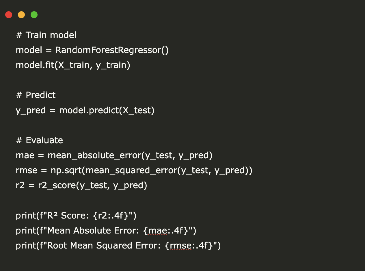
# Train model
model = RandomForestRegressor()
model.fit(X_train, y_train)

# Predict
y_pred = model.predict(X_test)

# Evaluate
mae = mean_absolute_error(y_test, y_pred)
rmse = np.sqrt(mean_squared_error(y_test, y_pred))
r2 = r2_score(y_test, y_pred)

print(f"R² Score: {r2:.4f}")
print(f"Mean Absolute Error: {mae:.4f}")
print(f"Root Mean Squared Error: {rmse:.4f}")
Configuration of an explanator
We have configured a tabularexplainer using the Shapiq package to calculate the Shapley interaction values based on the K-SII method (Shapley interaction index of order K). By specifying max_order = 4, we allow the explanator to envisage interactions of up to 4 features simultaneously, allowing more in -depth information on how the groups of functionalities have a collectively impact on the predictions of the model. Discover the Complete codes here
# set up an explainer with k-SII interaction values up to order 4
explainer = shapiq.TabularExplainer(
    model=model,
    data=X,
    index="k-SII",
    max_order=4
)
Explain a local body
We select a specific test instance (index 100) to generate local explanations. The code prints true and predicted values for this body, followed by a ventilation of its functionality values. This helps us to understand the exact entries transmitted to the model and defines the context of interpretation of the explanations of Shapley interaction that follow. Discover the Complete codes here
from tqdm.asyncio import tqdm
# create explanations for different orders
feature_names = list(df(0).columns)  # get the feature names
n_features = len(feature_names)

# select a local instance to be explained
instance_id = 100
x_explain = X_test(instance_id)
y_true = y_test(instance_id)
y_pred = model.predict(x_explain.reshape(1, -1))(0)
print(f"Instance {instance_id}, True Value: {y_true}, Predicted Value: {y_pred}")
for i, feature in enumerate(feature_names):
    print(f"{feature}: {x_explain(i)}")
Analyze interaction values
We use the Explain. Explain () method to calculate the Shapley interaction values for a specific data instance (X (100)) with a budget of 256 model assessments. This returns an object interaction, which captures how individual characteristics and their combinations influence the output of the model. The max_order = 4 means that we consider the interactions involving up to 4 features. Discover the Complete codes here
interaction_values = explainer.explain(X(100), budget=256)
# analyse interaction values
print(interaction_values)
First -order interaction values
To keep things simple, we calculate the first -rate interaction values – ie, standard Shapley values which only capture contributions from individual characteristics (no interactions).
By defining Max_order = 1 in the TreeExplanter, we say:
“Tell me to what extent each functionality contributes individually to prediction, without considering the interaction effects.”
These values are known as Shapley's standard values. For each characteristic, he considers the average marginal contribution to prediction in all possible permutations of the inclusion of characteristics. Discover the Complete codes here
feature_names = list(df(0).columns)
explainer = shapiq.TreeExplainer(model=model, max_order=1, index="SV")
si_order = explainer.explain(x=x_explain)
si_order
Draw a cascade graphic
A cascade graph visually decomposes the prediction of a model into contributions from individual functionalities. It starts from the basic prediction and adds / subtracts the value of Shapley from each feature to reach the planned final outing.
In our case, we will use the outing of TreeExplainer with max_order = 1 (i.e. individual contributions only) to view the contribution of each functionality. Discover the Complete codes here
si_order.plot_waterfall(feature_names=feature_names, show=True)
In our case, the reference value (that is to say the expected output of the model without any functionality information) is 190.717.
As we add the contributions of individual characteristics (Shapley Order-1 values), we can observe how each pushes the prediction up or pulls it down:
- Characteristics such as weather and humidity have a positive contribution, increasing the prediction above the basic line.
- Characteristics such as temperature and year have a strong negative impact, respectively reducing the prediction of −35,4 and −45.
Overall, the cascade table helps us to understand what characteristics stimulate prediction and in which direction – providing a precious overview of the decision -making decision.
Discover the Complete codes here. Do not hesitate to consult our GitHub page for tutorials, codes and notebooks. Also, don't hesitate to follow us Twitter And don't forget to join our Subseubdredit 100k + ml and subscribe to Our newsletter.

I graduated in Civil Engineering (2022) by Jamia Millia Islamia, New Delhi, and I have a great interest in data science, in particular neural networks and their application in various fields.